Mixed Precision Training for Machine Learning (Part I)
When training your deep learning models, one major concern is training time. Today we summarize a method which leverages your hardware when training models with a large number of parameters, in order to achieve a speed boost. This approach is called mixed precision training and is based on the seminal joint paper Mixed Precision Training1 by Baidu and NVIDIA researchers.
Precision Formats
In machine learning and computing in general, more often than not that we must do computations outside the realm of integers. However, since most real numbers are irrational and our computers have finite memory, we can never represent a real number exactly on a computer.
Therefore computer engineers have developed hardware around the convention that we will store a real number up to a certain number of significant digits (in binary), and each significatn digit is stored as a bit in memory. We will soon touch on terms such as float32 and float16.
Representing a number in binary
Our familiar number system uses base 10, i.e. we use the convention of representing every number as a sum of powers of 10, i.e.
\[12.45 = 1 * 10^1 + 2 * 10^1 + 4 * 10^{-1} + 5 * 10^{-2}\]In binary the same number is represented as
\[12.45 = 1100.01110011001 = 10^4 + 10^3 + 10^{-2} + 10^{-3} + 10^{-4} + 10^{-7} + 10^{-8} + 10^{-11}\]Since now we use powers of 2 instead of powers of 10, the only possible digits are 0’s and 1’s. Each binary digit is also called a bit. Already we notice that representing a number in binary instead of decimal yields more significant digits.
Single precision
One convention we use for storing (an approximation) of real numbers on a computer is single precision or float32. This means that we will use 32 bits of memory to represent a number. However, this doesn’t just mean we shove 32 significant digits in there. Each bit serves a very specific purpose.
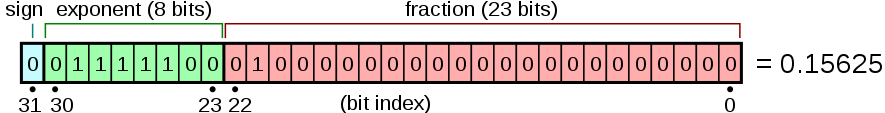 Image from Wikipedia 2
The first bit \(s\) is the sign, it stores whether the number is negative or positive. The next 8 bits store the exponent \(\epsilon\) in binary. The remaining 23 bits store the significand, call this \(b = (b_1, \cdots, b_{23})\). The number associated with these 32-bits is given by
\((-1)^s \cdot 2^{\epsilon - 127} (1 + b)\).
Let’s calculate the range of such a configuration. The maximum and minimum exponents are 255 and 0 respectively, so with the offset of -127 we have a max value of \(128\) and minimum value of \(-127\) for the exponent bits. However the maximum and minimum exponents are reserved for special numbers. So the actual max and min exponents we can use are \(127\) and \(-126\) respectively. For the significand, the maximum value is \(1 - 2^23\). With a plus sign in front, we get that the maximum possible value is
\[2^{127} (2 - 2^{23}) \approx 3.4028235 * 10^{38}\]with the minimum possible value the negative of that number.
For precision, the smallest positive number is \(2^{-149} \approx 1.4 * 10^{-45}\) and the biggest negative number is the negative of that.
This range is good enough for almost all computational purposes.
As for the reserved special numbers, those have to do with overflow, underflow, and indeterminates. A very nice summary of floating point is given in these course notes.
Half Precision
Half precision or float16 uses 16 bits: 1 for the sign, 5 for the exponent, and 10 for the significand.
This format results in a smaller range and more coarse precision than both single and double precision. Positive numbers range from \(2^{−24} \approx 5.96 * 10^{-8}\) to \((2 - 2^{-10}) * 2^{15} = 65504\).
Double Precision
There is another format called Double precision, or float64. Here we use 64 bits: 1 for the sign, 11 for the exponent, and 52 for the significand.
Tradeoff
Here we can see a tradeoff between the amount of memory used and the precision of the computation we are doing. The more precise we make our calculations, the more memory we need to use and vice-versa. Moreover, since we are using less digits, we also speed up computation time. For machine learning, we would obviously like to achieve the dream of using low memory to achieve high precision.
At first this seems like a logistical problem: How can we allocate more memory? How can we reduce the number of parameters in a deep neural network? But it turns out that we can exploit a bag of tricks of floating-point arithmetic we achieve our dream scenario.
The idea (and the tricks)
To fully explain the idea, let us first think about what kind of arithmetic operations are done when we train a neural network. No matter what the type of network it is, be it fully-connected, convolutional, or recurrent, the main operations are one of the following: matrix multiplication, reduce operations (e.g. summing up all entries of a vector, mostly comes up when computing means), or activation functions.
In the old days we carried out all these operations in float32. Now that we realized float16 saves memory and speed, we would ideally like to carry out all these operations in float16.
However, a potential pitfall is the significant loss in precision. Consider the following float32 : \(2^{-16} = 0 01101111 00000000000000000000000 \approx 0.00001525 = 1.525 * 10^{-5}\). I have written the 32-bit representation on the right, but clearly since the exponent is -16, it cannot be represented as a float16 number. Which means that such numbers will be treated as 0 in float16. And of course as we know, quantities to the scale of \(10^{-5}\) or smaller is very common in machine learning (small learning rates, small gradients, etc.). In fact, experiments have shown that over half of activation gradients involved in training certain models are too small to be represented by float16 numbers, and therefore get rounded down to 0.
Coupled with the fact that each pass through the neural network involves potentially millions of arithmetic operations, a seemingly small error such as this can compound into bigger errors. Ultimately affecting model accuracy. So the key idea is to identify when exactly we can get away with using float16 instead of float32. Let’s use base-10 to give some examples.
- Addition: Does not affect precision, if we add two numbers in base-10 with 2 significant digits for example: \(1.43 + 55.09\), the result still has at most 2 significant digits. Likewise, adding 2 float16’s stays in float16.
- Multiplication: Of course when we use float16 to multiply, every language we use that supports float16 will give us the product back in float16. So it may seem like multiplication doesn’t change precision either, but there is secretly a casting operation done under the hood. Again let us consider a base-10 example: \(0.2 * 0.3 = 0.06\). The multiplicands both had 1 significant digit but the product now has 2. If we were hypothetically working in the world of float1’s, allowing only 1 significant digit, then we will have to get rid of the 6 digit somehow. Depending on the implementation it could be rounding-up or rounding-down. Either way some precision is lost here.
Trick 1: Master Copy
The mixed precision approach keeps a master copy of the weights in float32, with the float16 conversion being used in the actual model.
What this means is that in the beginning, before the first pass through the model, the weights are initialized in float16 and a float32 master copy is then copied from the initial weights are stored separately. Then before each forward and backward pass, the weights are converted from the master copy into float16 and used for the model (this has no effect for the first training iteration but has an impact later on). After carrying out all relevant computations in float 16 (with performance improvements outlined in the next 2 tricks), the weight update is done in float32 on the master copy.
In other words, we use float16 copies of the weights purely as a funnel for time-saving computations, whereas the actual weights we store for the model are in the float32 master copy. This ensures that we don’t lose precision.
But what about the precision lost when converting from the master copy into float16? Let’s do an example in base-10 to see what happens:
Consider doing gradient descent on the convex function \(f(w) = w^2\) with learning rate \(0.0001\), starting from the initialization \(w = 1\). Initially the weight \(w = 1\) is stored in “float2” and a master copy is made in “float6” (*). After calculating gradients, we get that we should subtract \(2 * 0.0001 = 0.0002\) from the weight for the update (note that the weight updates are in the higher precision). This leaves us with the new weight being \(0.9998\). So far so good.
For the next iteration, the weight \(0.9998\) gets cast down to \(0.99\) before gradient computations, then the gradient would be \(0.99\) and the weight update is given by \(- 0.000198\). After updating, the new weight becomes \(0.999602\). But in the cast iteration the weight gets cast down to \(0.99\) again! So it seems like we got stuck in a local minimum with the weights.
However, we did get a nonzero gradient in the previous iteration, namely \(- 0.000198\), and the weight is continually being updated in the master copy. Which means that after more iterations, the master copy will eventually become \(0.98...\), and the “float2” version of the weight will change to \(0.98\), then \(0.97\), and so on, until \(f(w)\) reaches the global minimum of \(w = 0\).
Trick 2: Loss Scaling
We briefly mentioned that most of the activation gradients during training are too small to be represented by float16. However, it is rare to see huge gradients and loss functions(to the order of \(> 2^{12}\)). This means that we can preserve all the information of a float32 gradient in a float64 format simply by shifting bits!.
The procedure is as follows:
- Compute loss function in float32
- Convert loss value to float16 by shifting bits up.
- Backpropagate with the float16 loss value, notice that by the rules of differentiation, the (constant) scaling is preserved in this step.
- Scale the bits back down into float32.
- Do gradient clipping, weight decay, etc. (optional)
The final gradient will be in float32 after this procedure, but we have saved a lot of computation time during the computationally intensive backpropagation phase. Moreover, we don’t lose any precision by doing this!
How is the scaling factor determined? A very simple trial-and-error approach: we start with the largest possible factor \(2^{15}\) and check if the result overflows, if it does then we drop the scaling factor by a factor of 2, and so on until overflow no longer happens. The authors of the paper have found that a scaling factor of \(2^3\) (3 bits) is good enough for most purposes.
Trick 3: Arithmetic Precision
In the training of neural networks, we often need to multiply matrices. When multiplying two matrices \(A_{m \times n} \cdot B_{n \times k}\), the \((i, j)\)-th entry of their product is given by \(\displaystyle\sum\limits_{\ell=1}^n a_{i, \ell} b_{\ell, j}\). Notice that such a computation consists of a series of scalar products added together.
As we have seen earlier, float16 numbers naturally multiply to float32 numbers. The strategy in the paper is to store the scalars of the matrices in float16, then when they are multiplied, keep them in float32 until all the addition operations are done, and only then cast them back to float16.
To see the upshot of this approach, let us again consider an example in base-10. We want to compute the quantity \(1.23 * 0.45 + 2.12 * (-5.94)\). These scalars are stored in “float2” at present. The result ends up being \(-12.0393\), which has 4 significant digits (in the real world).
Let us first carry out the usual computation of our computers in “float2”, which is to multiply into a “float4” number and then cast down to “float2” immediately. Then we get \(0.5535 + (-12.5928)\), each of which gets casted down to \(0.55 + (-12.60) = -12.05\).
Now let us accumulate the sums in “float4” before we cast back down. By using the round-down convention, we get \(-12.04\) when we convert back to “float2”. This means that accumulating the sums before casting back down preserves higher precision. This effect becomes compounded when the matrices are very large, resulting in more addition operations.
Conclusion
The authors note that training models with mixed point precision has accuracy comparable to training in float32, with the added benefit of saving computation time for many models.
In the next post in this series, we will talk about how to implement mixed precision training using Pytorch.
(*) It should be noted that the base-10 examples are purely for demonstration, and that the terms “float2”, “float4”, and so forth are meaningless for the floating point arithmetic of most CPU architectures, which are in binary. And of course, float32 does not mean that the maximum precision is exactly 32 digits for each number, since numbers can go as low as \(2^{-149}\).
-
Micikevicius, P.; Narang, S.; Alben, J.; Diamos, G.; Elsen, E.; Garcia, D.; Ginsburg, B.; Houston, M.; Kuchaiev, O.; Venkatesh, G. & Wu, H. Mixed Precision Training (2017) ↩
-
https://en.wikipedia.org/wiki/Single-precision_floating-point_format ↩